Building Langflix's Recommendation System with a Two-Tower Model

Hello! I'm Jaewook Yeo, and I worked with Theta One on Langflix's recommendation system from July to August 2026.

I was primarily responsible for the Two-Tower model that recommends Shorts to warm users based on their interests. In brief, we grouped all Shorts into 50 clusters, represented users and items in the same embedding space using viewing history, and compared the two vectors for similarity.

Put simply, we embedded users close to videos they liked and farther from those they disliked or showed little interest in. We could then recommend other unwatched videos near that user.

For a first version, the features were relatively simple: viewing history and video text. The model itself was a compact multilayer perceptron. This post focuses less on the model architecture than on the questions we had to answer before building it.

We had to consider both the goal of a learning app and the need for lightweight, real-time serving. I'll start with raw viewing records and explain, step by step, how we designed features and models and finally served recommendations.

1. What makes Langflix recommendations different?​

The first step was understanding Langflix's goals and constraints.

Langflix helps people learn English words and expressions using Netflix and YouTube Shorts. Unlike a general video recommender, its goal is not simply to surface clips that hold attention.

For a typical Shorts platform, one more view or one more second in the feed might be the goal. At Langflix, it mattered more that watching a Short led naturally to an actual learning action in the app.

Improving app retention was the overall project goal. Within the recommender, we aimed to increase use of learning features through Shorts. That aim later shaped our learning signals.

Free users could watch only three Shorts per day, while paid subscriptions were central to the business model. The two groups therefore needed different recommendation priorities.

Free users had few exposures and were usually in a cold-start state, making personalization difficult. Each limited exposure needed to show them the product's features and learning experience. We chose a pool of proven videos that many users had watched and that frequently led to learning actions, supplemented with onboarding survey answers.

Paid users generally had more behavioral history. For them, personalization could help sustain interest. We designed a model that inferred preferences from behavior and found matching videos, including less-viewed videos whose content suggested a good fit.

The old recommender relied heavily on popularity. Videos with many prior responses kept being shown; videos with few or no exposures kept falling behind. About 60% of all Shorts had received no exposure in the previous month. A traditional collaborative-filtering model based mainly on interactions would have struggled to recommend those cold items too.

We needed to reflect users' tastes while still recommending items without prior responses.

Finally, the model had to work in production. The Shorts tab scrolls indefinitely, so latency and memory mattered. The TypeScript server had to respond quickly without running a heavy Python model or applying a complex neural network to thousands of videos for every request.

The learning objective, cold-item problem, personalization, and real-time serving requirements all shaped the design.

2. Understanding user behavior​

Before recommending Shorts by taste, we had to decide what user behavior meant "I liked this."

Our first idea was to combine behaviors into a proxy for retention, the project's north-star metric. Retention matters, but measuring D1 or D7 after a model change takes days, and using whether a user returned as a direct training label would be inaccurate for several reasons.

We examined how directly observed behaviors related to retention and tried to identify stronger and weaker signals. In one experiment, we used the rates of learning-related actions to predict D1/D7 retention with logistic regression. We applied Bayesian smoothing to each user's action rates and normalized regression coefficients to use as potential behavior weights.

Initially, watching at least 50% of a video had the largest coefficient. Review, bookmarks, and repeat viewing also had smaller but meaningful coefficients. We considered combining them into one meaningful-action index.

But retention is affected by many factors and some chance. A handful of actions did not predict it reliably enough. ROC-AUC and checks for monotonicity between the index and retention showed clear limitations. We decided the coefficients were not trustworthy enough to use directly as a training signal or a single index.

The experiment still helped us understand which actions were relatively important and more closely associated with retention. Rather than build one proxy metric from exact coefficients, we used them alongside each action's frequency to identify a set of meaningful learning behaviors. The proxy metric failed, but the exercise was useful exploratory analysis.

3. Defining learning signals​

Langflix has no explicit rating such as stars, so we had to infer preference from behavior. We defined training signals from implicit feedback.

We classified four actions as meaningful learning: review, shadowing, listening, and saving expressions. We then assigned approximate interaction scores based on positive or negative direction and strength:

• +2: A learning action within a Short
• +1: Watched at least half the video or at least 20 seconds
• -1: Skipped within five seconds
• -2: Clicked "Not interested"
• 0: None of the above

The intended order was learning action > engaged viewing > neutral response > quick skip > explicit rejection.

A learning action after watching was a strong positive signal (+2). Watching at least half or 20 seconds without a learning action was a weaker positive (+1), suggesting interest in the topic or content. Skipping within five seconds was a weak negative (-1), and an explicit rejection was a stronger negative (-2).

We converted each user's responses to items into scores and built a user-item interaction matrix. Those interactions became the main basis for user features.

4. Building the Two-Tower model​

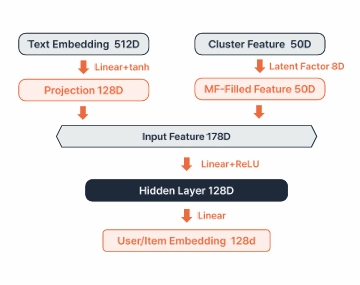
We chose a Two-Tower model because the information available to us was mostly video text and user activity history. We wanted a hybrid that used both collaborative-filtering and content-based information.

Collaborative filtering based only on user-item interactions can work well for items with sufficient history, but many of our items were cold. To recommend videos with no interactions, we needed their content too. A graph-based model would have been very sparse because each user had few interactions. A sequence model was also less suitable: users watched few Shorts in a day or session, so cumulative taste seemed more useful than the most recent viewing order.

Two-Tower represents user behavior and item content as features in a shared embedding space. Crucially, it learns a function that transforms item features rather than just learning an embedding for each item ID. A new Short can enter the same space using only its text and cluster information, even with no viewing history.

We could also compute item embeddings ahead of time. During training, the item tower transforms all item features into 128-dimensional embeddings, which we store. At recommendation time, we build the user feature, run the user tower once, and take dot products with the stored item vectors. The expensive work happens before serving, leaving a fast comparison when Langflix needs the next Short.

We kept this first version's features explainable and simple. Items used cluster assignments and text semantic vectors. Users used user-cluster interactions and semantic vectors from recently viewed videos. Each tower's MLP transformed those features into a common 128-dimensional space. We could later test channels, difficulty, sequences, and other features instead of adding them all at once.

5. Building item features, including difficulty​

Item features needed to capture each video's topic and content. Text was the most reliable information available. Images and audio were possible, but we left them out of the first version because of extraction costs and system complexity.

After comparing several embedding models on subtitles, we used three fields in the final implementation: title, subtitles, and synopsis. OpenAI's text-embedding-3-small turned each into a 512-dimensional vector. We combined them with weights of 0.4 / 0.5 / 0.1 respectively.

Titles briefly identify topics or people; subtitles directly capture what is said. Synopses add context but often include social links and promotional noise, so we gave them the least weight.

We mean-centered and L2-normalized the resulting semantic vectors, then grouped them into about 50 clusters with Spherical K-Means. At first, we considered a one-hot hard assignment to one cluster per video. But an interview with a celebrity might also discuss relationships or self-improvement. One topic could not always describe it.

We instead assigned up to three nearby clusters, weighted by similarity and normalized to sum to one. That produced a 50-dimensional soft cluster feature. Joining it to the 512-dimensional text vector gave us a 562-dimensional item feature.

Difficulty was different from taste​

We suspected difficulty would matter as much as topic. Users could watch Shorts on YouTube; choosing Langflix suggests they also want to learn English. A video therefore needs to suit their current learning level, not merely their interests.

We distilled difficulty into three dimensions:

• CEFR level of vocabulary in the video
• Average word length
• Speaking speed estimated from subtitle timing

We normalized these measures and converted them into one difficulty_score and five difficulty buckets. Initially, we considered feeding difficulty into the Two-Tower model. But topic preference is continuous, whereas avoiding the hardest video for a beginner is closer to a constraint. We used difficulty as a prefilter when forming candidates, comparing it with the user's onboarding English level to exclude videos that were far too easy or hard.

6. Building user features, including matrix factorization​

To complement item features, we represented users in two matching ways.

First was a semantic text profile describing the content they had recently liked. We took the 512-dimensional text embeddings of up to 30 recently viewed Shorts and formed a weighted average. Rather than averaging equally, we weighted each video by the interaction score defined earlier: a +2 response pulled the profile strongly toward a video, while a quick skip pushed it away.

We also applied time decay. A recent video is more likely to reflect current interests, so the i-th earlier video received a weight roughly proportional to exp(-0.05i). Recent, strongly positive videos mattered most, while older ones gradually mattered less. For users with very little history, we scaled down the profile's influence so a handful of views would not determine its direction too strongly.

The second feature summarized the user's response to each content cluster. A user-item matrix across roughly 5,000 items was mostly empty because most users had watched fewer than 30 videos. We grouped items into the 50 clusters described earlier and aggregated interaction scores within each cluster to form a user-cluster matrix.

For example, if a user's responses to cluster 3 were +1, +1, 0, +2, +1, -1, we summed and bounded them to represent that user's preference for the cluster. But even with 50 clusters, individual users had not encountered every cluster, leaving gaps.

We used matrix factorization to fill them approximately. We decomposed the user-cluster matrix into:

• A global mean
• User bias
• Cluster bias
• User latent factors
• Cluster latent factors

We trained these components to reconstruct observed interactions. The final version used eight-dimensional latent factors with mean squared error loss. Combining the trained components let us estimate a response for a cluster a user had never seen: "Given this user's reactions to other clusters and other users' behavior, they might like this cluster about this much."

The resulting user feature joined a 512-dimensional profile of recently viewed video text with 50-dimensional cluster interactions made less sparse by matrix factorization. One captures detailed semantic taste; the other captures preference for broader content topics.

7. Designing the loss function​

With user and item features in place, we needed a criterion for arranging their embeddings. Our main loss was Bayesian Personalized Ranking (BPR). For recommendations, predicting an exact absolute score is often less important than ranking video A above B when a user prefers A.

We trained on pairs so high-scoring items would sit closer to the user than low-scoring ones. Because BPR focuses on relative order, we added Smooth L1 as an auxiliary loss to maintain some relationship between interaction scores and model similarities.

Negative sampling was more difficult than the loss formula. A video someone never watched is not necessarily disliked; the old recommender may simply never have shown it. Treating every unseen item as negative would further disadvantage the many cold items we were trying to surface.

We distinguished observed negative responses, such as quick skips, from unexposed items. We included some unseen items in training but gave them much less weight than observed negatives and limited their number relative to positives. Users with negative responses but no positive interaction were excluded from BPR training. We also adjusted per-user loss contributions so a few highly active users would not dominate.

What counted as positive or negative, and which pairs we trained on, mattered as much as the model architecture.

8. Producing the final ranking​

A Two-Tower similarity score alone did not determine the ten videos we showed. We first filtered out recently viewed or exposed videos, excluded content, blocked channels, and videos far above or below the user's English level.

Then we computed dot products between user and item embeddings and retrieved the top 100 Two-Tower candidates. We also brought in popularity candidates. Two-Tower reflects personal taste but can rank untested content highly; popularity offers reliably well-received content. Our popularity signal used learning actions over the last 30 days rather than raw views, and we admitted only items with a minimum Two-Tower score so they would not be completely unrelated to the user's interests.

We applied maximal marginal relevance (MMR) to avoid showing similar videos back to back. It prioritized relevance to the user while penalizing items too similar to those already chosen for the feed. We measured video similarity using the text embeddings and capped how many items could come from the same cluster.

Finally, epsilon-greedy exploration reserved some slots for items that neither Two-Tower nor popularity consistently selected, so they could gather new interactions. The final feed therefore passed through candidate filtering, Two-Tower and popularity retrieval, MMR reranking, and exploration.

9. Offline evaluation​

Once the model worked, the hardest question was how to decide whether it was good. Recommendation systems commonly use Recall@K and nDCG@K, but Langflix's historical interactions came from a popularity-driven recommender. If the old model mostly exposed popular videos, the test set would also contain many popular videos. A model that copied popularity could achieve high Recall, while one that discovered cold items could score worse.

Finding good cold items was one reason we built Two-Tower. We therefore evaluated four additional offline metrics matched to our goal instead of choosing a model by Recall or nDCG alone.

Embedding Effective Rank checked whether the 128-dimensional outputs occupied diverse directions rather than collapsing into just a few. The final model's effective ranks were about 12.06 for user embeddings and 25.03 for item embeddings.

Cold Coverage@5 measured the fraction of all cold items recommended at least once when giving every evaluation user five items. During training, about 58.8% of items were cold. The final model achieved 12.02% Cold Coverage@5.

Ordinal Accuracy compared pairs of items that appeared in the test data and checked whether Two-Tower gave the higher score to the item with the higher observed interaction score. Its ordinal pair accuracy was 0.644, or the correct preference order for about 64.4% of pairs.

Cold Recall@5 focused on items that were cold in training but received positive user responses in the test period. It asked whether the model could have recommended them before they had interactions. On a seven-day test set, Cold Recall@5 was 3.65%.

Together, these metrics checked for collapsed embeddings, exploration of neglected items, learning of relative preference, and discovery of promising cold items. The exercise showed me that evaluation criteria must reflect both a service's goal and how its data was generated.

10. Serving the model and storing data​

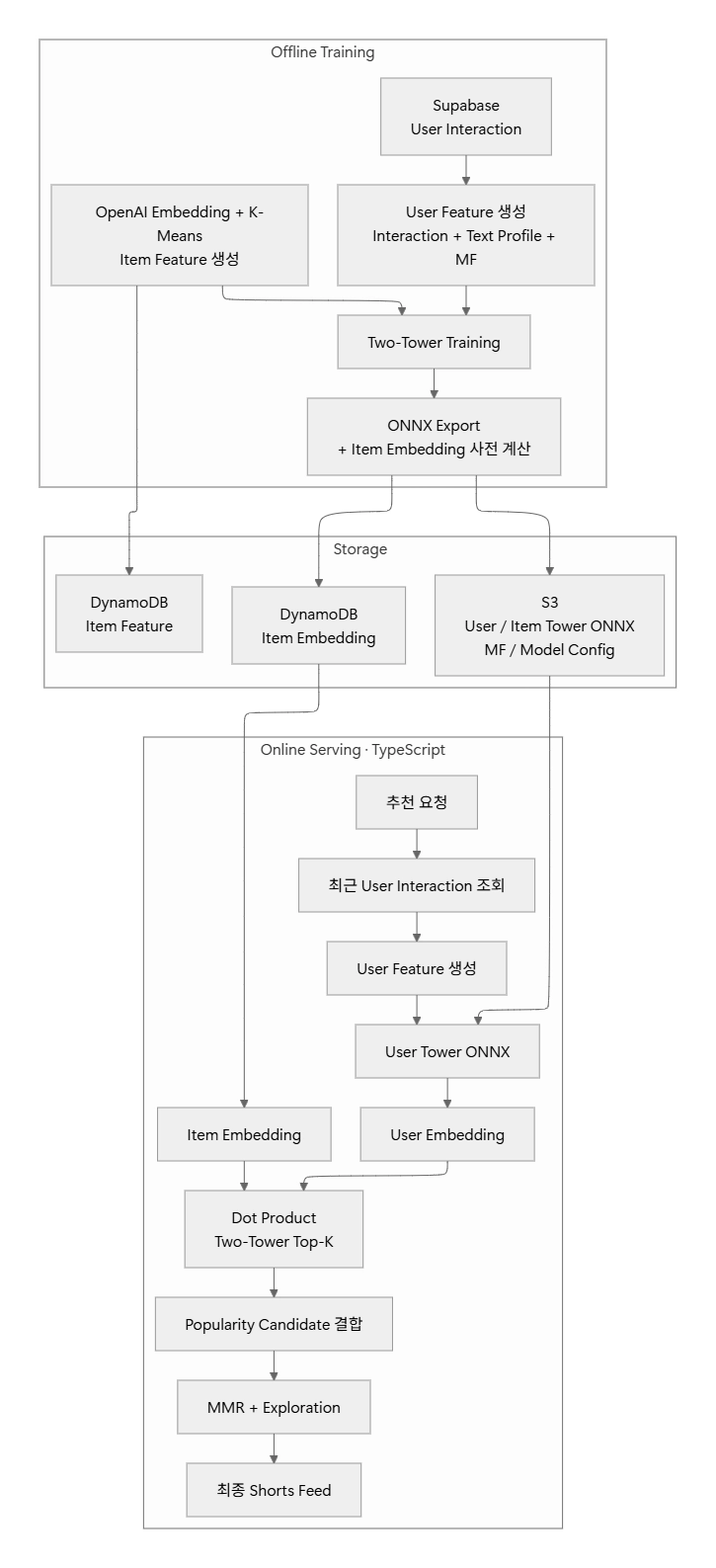
A model that runs in Python is not automatically ready for production. Langflix handled recommendation requests in a TypeScript server, so we separated training from serving.

At regular intervals, training read user interactions, trained matrix factorization and Two-Tower, exported both towers to ONNX, and precomputed and stored all item embeddings.

A new Short did not require retraining the entire model. We could create its text embedding and cluster assignment, assemble its item features, and run the existing item tower once to generate its embedding. An item with no behavioral data could immediately become a candidate using its content alone.

During serving, we fetched recent interactions, built user features, ran the user tower once, and took dot products with stored item vectors. We then retrieved Two-Tower and popularity candidates and applied MMR to return the ranking. For a user near the P99 workload, we estimated an end-to-end recommendation time of about 59–79 ms, meeting our real-time target.

We separated storage by purpose. Supabase held interactions and source content; DynamoDB held item features and embeddings needed quickly at serving time; S3 held model artifacts such as ONNX files, matrix-factorization state, and model configuration.

We versioned text embeddings, cluster centroids, item embeddings, and towers together to prevent incompatible artifacts from being used at once. A new model became active only after every artifact was generated and validated; if something failed, the previously healthy version remained in use.

Building a recommendation system meant connecting raw data, features, training, artifact storage, new-item handling, and online serving, not merely training one model.

11. Hyperparameter tuning and experiments​

After the first Two-Tower version ran, we spent more time diagnosing odd recommendations and fixing them one by one than adding new architecture.

One early issue was item embeddings pointing in similar directions. We initially used ReLU, but suspected removing the negative range contributed to that collapse. We switched to tanh and checked effective rank and embedding distributions. We also tried centering regularization to keep mean embeddings near the origin, but strong regularization interfered with personalized ranking, so we left it out of the final model.

More epochs did not always help. Repeatedly training on sparse interactions caused overfitting, so we substantially reduced updates. We tried several matrix-factorization ranks and lowered the latent dimension from 16 to 8. We also adjusted quick-skip strength and the number of negative samples so negative feedback would not dominate user vectors.

We explored positioning cold items near similar warm items in embedding space, but prioritized improvements to Two-Tower's content features, negative sampling, and exploration. We tried a multi-behavior model with separate representations for learning and ordinary viewing, but it did not consistently beat the single representation on our data, so it was excluded.

At the start, I expected more features and layers to improve the model. In practice, simpler choices often worked better: changing the activation, training for fewer epochs, reducing matrix-factorization dimensions, limiting negative samples, and removing structures with unclear benefits. The final model was a relatively small Two-Tower whose features and losses we could explain and serve in production.

12. Limitations and future work​

Within a limited project period, we focused on a first version that could actually run in the service. We worked across interaction definitions, feature engineering, training, offline evaluation, and serving, but could not test every idea thoroughly.

The current model gives each user one embedding, although interests can point in several directions. I would like to test multi-interest embeddings and separate representations for learning and general viewing more thoroughly. Some experiments did not show a stable improvement over the existing structure and were not included.

We also used roughly the same MMR diversity weight and difficulty filters for most users. With more data, we could tune diversity differently for users who focus on one topic versus those who explore many, and adapt difficulty per user based on actual learning actions.

The proxy metric we tried early on might also improve with more data. Rather than compress everything into one interaction score, we could predict probabilities for sufficient viewing, saving expressions, review, and shadowing separately, then combine them according to the learning value Langflix assigns to each behavior.

My biggest regret is that we could not run the Two-Tower online A/B test long enough. We designed offline metrics to account for the old popularity recommender's bias, but only actual learning behavior and retention can ultimately tell us whether recommendations are better.

Next time, I would want a full feedback loop: offline evaluation → exploration → online experiment → new interaction data → retraining. What we produced is less a finished recommendation algorithm than a first end-to-end structure for deciding which signals to use, how to represent and train users and items, how to evaluate them, and how to connect the result to the service.

13. Results and reflections​

We designed the recommendation model with teammates almost from scratch and thought through how to make it work in actual production code. Alongside general recommendation challenges, we had to account for Langflix's goals and operational constraints. The work involved many discussions, research, and learning with AI assistance.

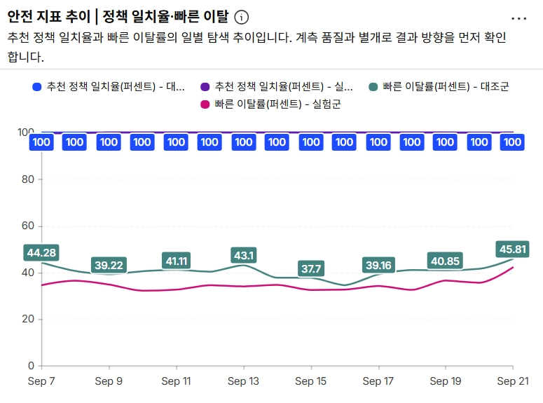
In our late-project A/B test, the treatment group using our recommender showed a somewhat higher effective learning-action rate per video than the control group using the old system. The test was too short and too small for a statistically significant conclusion. Still, the target metric did not deteriorate and moved in a promising direction, and we created the groundwork for a longer online experiment.

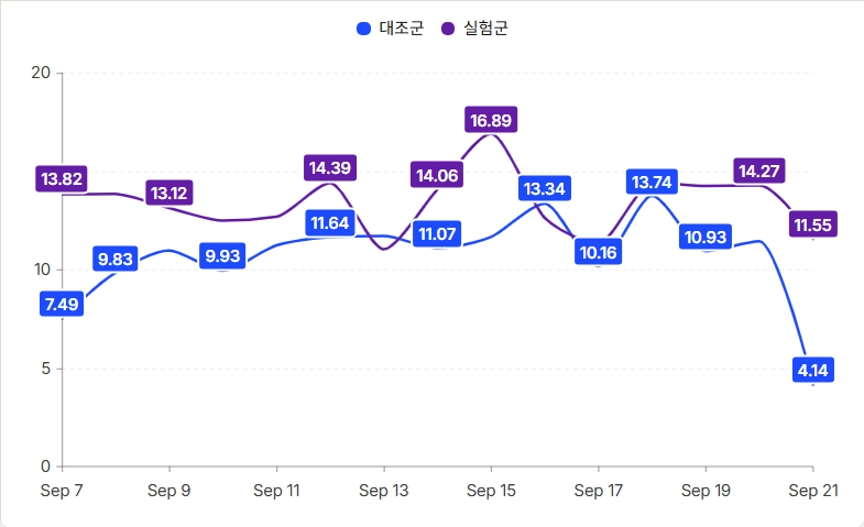
We also monitored guardrail metrics such as quick exits to check whether personalized recommendations harmed the user experience.

The aim was not to build the most complicated model, but a first recommender suited to Langflix's data, product goal, and serving environment. Connecting an offline model to the service and observing real user responses was the most meaningful result for me.

I especially valued learning the development work needed to put a machine-learning model into production. AI agents helped me understand an unfamiliar TypeScript codebase, learn the necessary structures and libraries, and implement recommendation serving. More than generating code, they helped me learn new technology quickly, check what I built, and revise it.

I also experienced GitHub collaboration through branches, commits, and pull requests; experiments in PostHog; user logs in Supabase; and model artifact design. Storing models and features in S3 and DynamoDB and connecting the service through ECS task roles showed me the entire path from ML model to production operation.

Growth Hackers and Theta One gave us opportunities to learn and grow together. I hope the model and work we contributed help Langflix reach more users and grow further. I'll be cheering Theta One on!